RTSF argues the linear map is not the weak part of long-term forecasting, sparsity is
Revisiting Long-term Time Series Forecasting: An Investigation on Linear Mapping
At a glance
- What is it?
- A simplified write-up of an arXiv paper that gives closed-form solutions for the transition matrix of a single linear layer on seasonal series, with a simulated sine wave as the worked example and an explicit admission that long input horizons make the optimisation hard because the matrix is sparse.
- Who is it for?
- Read RTSF as an argument rather than as a library, because what it delivers is notation and closed forms that let you reason about the linear baseline directly instead of treating it as a weak default. It is useful if you are choosing between a plain linear model and something heavier, since the theorems explain why a single layer can be competitive on seasonal data and the limitations section is honest about where that stops.
- Can I use it commercially?
- Not without permission. GitHub finds no licence file in the repository, and without a licence all rights are reserved by default: you may read the code but not reuse it. Check the README, or ask the authors, before using it.
- Is it still maintained?
- Probably not. The repository last received commits 37 months ago, on September 13, 2023.
- What is it written in?
- Mainly Jupyter Notebook, according to GitHub's language statistics.
Answers come from the project's GitHub data, last synced on October 22, 2026, and from our analysis. They are not legal advice.
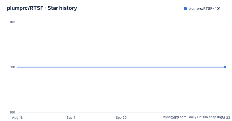
Star history
- plumprc/RTSF101 ★ · +0
| Repository | 2026-08-18 | 2026-10-22 |
|---|---|---|
| plumprc/RTSF | 101 | 101 |
0 Stars in the last 65 days, measured from the daily GitHub snapshot. Compare with other projects
Editorial analysis
The claim is that the linear map is not where forecasting fails
The whole argument fits in one line of algebra. Take a historical series X with c channels and n time steps, predict the next m steps Y, and require X and Y to be consecutive in the original data. The model class is a single linear layer, a weight W of shape n by m plus a bias b of shape 1 by m, applied to the input vector to produce the output vector. W is called the transition matrix, and that name is the thesis in miniature: the question the paper asks is not whether a linear map is expressive enough in principle, but how much of it you can write down in closed form. Every theorem in the README exists to construct that matrix for a particular kind of series. Where it succeeds, the answer is exact rather than fitted; where it fails, the failures are structural and are named rather than hidden.
Theorem 1 gives a closed form whenever the series is seasonal
The first result is the base case. Take a seasonal series satisfying x(t) = x(t - p), where p is the period and p is no larger than the input length n. The theorem states that an analytical solution for the linear model always exists, and the formula for it is sparse in an obvious way: entry W_ij at level k equals 1 when i equals n minus kp plus the position within the period, and 0 otherwise, for k running from 1 up to the floor of n over p, with the bias set to zero. Read plainly, each level k is a lag of k periods copied onto the output positions, and the matrix is a stack of shifted copies of the same row pattern. Since the bias is zero and the coefficients are ones, this is not an approximation of the series at all. It is a restatement of the periodicity as a weight matrix.
Corollary 1.1 handles a scaled and shifted series, and the bias stops being zero
Pure periodicity is a special case, and the corollary widens it to x(t) = a times x(t - p) plus c, where a is a scaling factor and c a translation factor. The structure of the matrix is the same shifted-copy pattern as in Theorem 1, but the entries at level k become a to the power of k rather than 1, and the bias becomes a cumulative sum from l = 0 to k - 1 of a to the power of l times c. That is the whole difference, and it is a meaningful one: a series that grows or decays geometrically each period no longer needs a fitted offset, because the offset follows in closed form from the same factor. Together the two results cover the case people usually meet in practice, where a daily or weekly pattern rides on a slow upward or downward trend.
Theorem 2 bounds the error without ever fitting the weights
The third result is the most general and the least intuitive. Decompose the series as x(t) = s(t) plus f(t), where s is a seasonal signal with period p and f is K-Lipschitz continuous. The theorem says there exists a linear model with an input horizon of n = p plus tau, for tau at least zero, such that the error at each future step j is bounded by K times (p plus j), for j running from 1 to m. Two things follow. The bound depends on the Lipschitz constant of the irregular part and on the period, and not on how well you have estimated anything. And the horizon need only be one period long, plus slack, which is a striking claim for a task where longer lookbacks are usually assumed to help. The cost is that K is a property of the residual you are handed rather than something the model can learn.
Theorem 3 needs the least common multiple, and that is where sparsity bites
The multivariate result is the one with a practical cost. If each channel of the input has its own period p_i, a linear model predicting the next m steps must exist once n is at least the least common multiple of all those periods. The limitation section is explicit about the consequence: an excessively long input horizon makes optimising W difficult because the matrix is sparse. The illustration uses an input horizon of 336 and a prediction horizon of 192, comparing RLinear with RLinear-CI, and the observation is that with CI different projection layers learned different periodic features and in more detail, while a single linear layer concentrates on global periodicity and is prone to forget fine-grained periodic features. The authors call balancing periodicity across scales a question for further work.
Any convex combination of the period solutions still works
The showcase is a simulated sine wave, y = sin(2 pi over 30 times x), so the period is 30, and the input length and the prediction horizon are both set to 90. Theorem 1 supplies three solutions, W to the first, second and third power, and the result worth noticing is that any linear combination of those three still satisfies the prediction conditions as long as the coefficients sum to one. In other words the family of valid solutions is not a single point but a simplex, so a fitted model is not fighting to find one blessed matrix; it is searching inside a set where every member is already correct. The README then draws the wider conclusion, that prediction based on periodicity is not sensitive to the form of the input data, and connects it to why a single linear layer does well on real datasets whose seasonality runs in days, weeks, months and years.
The repository ships the experiment code next to the exposition
It is not a document-only repository. At the top level there is run.py as the entry point for experiments, simulate.py for the synthetic setups the theorems are illustrated with, tutorial.ipynb as a notebook, script.md, and directories named models, layers, data_provider, exp and utils, plus a pics directory holding the figures the README embeds. That layout matches a paper repository rather than a released package, and it means the claims are at least partly reproducible from the tree if you are willing to read the code. There is no packaging metadata, no version and no install instructions in the README, so there is nothing to install; you clone it and read or run it in place. The primary language is recorded as Jupyter Notebook, which matches tutorial.ipynb being the entry point for most readers.
The underlying work is an arXiv preprint by four named authors
The citation block names the paper this repository condenses: Revisiting Long-term Time Series Forecasting: An Investigation on Linear Mapping, an ArXiv article from 2023 with volume abs/2305.10721, authored by Zhe Li, Shiyi Qi, Yiduo Li and Zenglin Xu, and the README links it at arxiv.org/abs/2305.10721. Questions go to [email protected]. The acknowledgements name three repositories for code or datasets, Informer2020 from zhouhaoyi, RevIN from ts-kim, and LTSF-Linear from cure-lab, which is where RLinear and the LTSF benchmark conventions come from. The repository itself is not archived and sits on main with a last push dated 2023-09-13, reports 101 stars, 8 forks and 2 open issues, and no licence is recorded for it, so treat reuse as something to check with the authors.
Editorial conclusion
Read RTSF as an argument rather than as a library, because what it delivers is notation and closed forms that let you reason about the linear baseline directly instead of treating it as a weak default. It is useful if you are choosing between a plain linear model and something heavier, since the theorems explain why a single layer can be competitive on seasonal data and the limitations section is honest about where that stops. Two cautions before you cite or reuse it. The complete proofs are not here, the README sends you to the original paper for those, so this is a summary of results rather than a source you can check a derivation against. And the repository is dated: the last push is 2023-09-13, no licence is recorded for it, and the underlying work is an arXiv preprint, so treat the claims as a preprint position rather than a settled one.
Frequently asked questions
What problem is RTSF actually solving?
Long-term time series forecasting with a single linear layer. Given c channels over n time steps, it predicts the next m steps with one weight matrix of shape n by m, called the transition matrix, and the paper's contribution is a set of closed-form solutions for that matrix on seasonal series rather than a new architecture.
When does the closed-form solution in RTSF stop working?
The multivariate case needs an input length at least equal to the least common multiple of the channel periods, and the README says an excessively long horizon makes optimising the matrix hard because it is sparse. With an input horizon of 336 and a horizon of 192, RLinear-CI learned finer periodic features that a single linear layer tended to forget.
Do I need the original paper to use RTSF?
For the proofs, yes: the README says to see the original paper for the complete proof and links it at arxiv.org/abs/2305.10721. What RTSF itself provides is the simplified statement of the problem, the four results, the sine wave showcase and the limitations, plus the experiment code at the top of the tree.
Official sources
Add this badge to your README
If you maintain this project, the badge below links readers to this analysis and shows its maintenance status from the daily GitHub snapshot. Paste the markdown into your README; add ?metric=license or ?metric=stars to the image URL for a different field.

[](https://hysenlabs.com/projects/plumprc-rtsf)Star history chart for your README
[](https://hysenlabs.com/projects/plumprc-rtsf)