gtsummary: publication-ready tables from R without hand-formatting every cell
Presentation-Ready Data Summary and Analytic Result Tables
At a glance
- What is it?
- gtsummary is an R package that turns data frames and regression models into formatted summary tables, most often a Table 1 for a clinical paper. It leans on gt for the output and, according to the README, computes every table from a structured Analysis Results Dataset so results stay traceable.
- Who is it for?
- gtsummary suits a statistician or analyst who publishes clinical or pharmaceutical results and wants a reproducible table rather than a spreadsheet copy, because the table is code, the formatting is declarative, and the README states results are computed from a structured ARD that survives review.
- Can I use it commercially?
- Check first. The repository uses a licence we do not classify automatically, so read its LICENSE file before any commercial use.
- Is it still maintained?
- Yes. The repository last received commits 11 days ago.
- What is it written in?
- Mainly R, according to GitHub's language statistics.
Answers come from the project's GitHub data, last synced on November 7, 2026, and from our analysis. They are not legal advice.
Star history
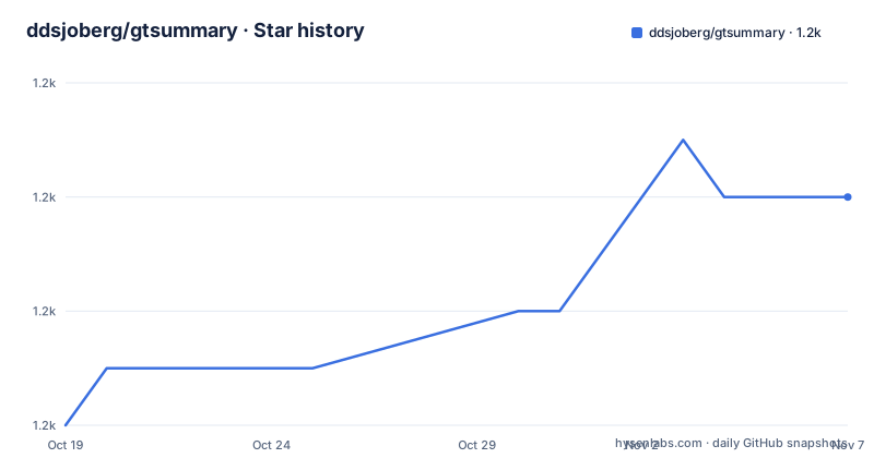
- ddsjoberg/gtsummary1,220 ★ · +4
| Repository | 2026-10-19 | 2026-11-07 |
|---|---|---|
| ddsjoberg/gtsummary | 1.2k | 1.2k |
4 Stars in the last 19 days, measured from the daily GitHub snapshot. Compare with other projects
Editorial analysis
One function replaces a page of formatting code
The {gtsummary} package provides an elegant and flexible way to create publication-ready analytical and summary tables using the R programming language, and the pitch is that a table comes out in a single line of code.
The mechanism is a pipeline of verbs. The core function is tbl_summary(), which takes a data frame and returns an object you can pipe further transformations into. The package leans on {broom} for tidying model output, {gt} for the actual table rendering, and {labelled} for variable metadata, and it was written as a companion to {gt} from RStudio, which is why the output object is a gt table with all of gt's formatting power behind it.
The default behaviour is the part that saves the most time. tbl_summary() automatically detects continuous, categorical and dichotomous variables in your data set, calculates appropriate descriptive statistics for each type, and includes the amount of missingness in each variable.
That last detail is not cosmetic. In a clinical table, whether the denominator is the non-missing count for one row and the total for another is the kind of inconsistency a reviewer will catch. Having missingness reported by default means the numbers that are present are also the numbers that are accounted for.
The audience is a statistician, analyst or clinical researcher producing a manuscript table, and the alternative they are replacing is either hand-built gt code or, far more often, a spreadsheet.
The Table 1 pipeline, in the README's own example
The basic usage is three lines.
library(gtsummary)

# summarize the data with our package
table1 <-
  trial |>
  tbl_summary(include = c(age, grade, response))
The customised version shows what the pipeline is for. Each step adds one thing, and the comments make the intent explicit.
table2 <-
  tbl_summary(
    trial,
    include = c(age, grade, response),
    by = trt, # split table by group
    missing = "no" # don't list missing data separately
  ) |>
  add_n() |> # add column with total number of non-missing observations
  add_p() |> # test for a difference between groups
  modify_header(label = "**Variable**") |> # update the column header
  bold_labels()
Three things are worth pulling out of that example. First, by = trt splits the table by treatment group, which is the actual shape of a clinical Table 1. Second, add_p() inserts a p-value test for a difference between groups, and add_n() adds the total non-missing count, so the two things a reviewer always asks for are one call each rather than a hand-written block. Third, the formatting verbs modify_header() and bold_labels() are pure presentation and sit at the end of the pipe, separated from the statistics.
That separation is the design. Statistical content is computed at the left of the pipe, presentation is applied at the right, and you can swap the presentation without touching the analysis.
Regression models with the right headers filled in
The second headline function is tbl_regression(), which turns a fitted model into a formatted results table.
mod1 <- glm(response ~ trt + age + grade, trial, family = binomial)

t1 <- tbl_regression(mod1, exponentiate = TRUE)
The README is specific about what the package handles here. Common regression models such as logistic regression and Cox proportional hazards regression are automatically identified, and the tables are pre-filled with appropriate column headers, meaning Odds Ratio for the logistic case and Hazard Ratio for the Cox case. Reference rows for categorical variables are included as well.
That is the practical win. Producing a regression table by hand means remembering to exponentiate the coefficients, remembering to express them as ratios rather than log odds, remembering the right column header, and remembering to add a reference level row for every categorical predictor. Each of those is a chance to produce a table that looks right and is subtly wrong.
Models are also composable. The README shows side-by-side presentation using tbl_merge(), so two models, for instance a univariable and a multivariable version, can sit next to each other with aligned rows. A survival example is included, using coxph with Surv(ttdeath, death) as the outcome, piped into tbl_regression() and then merged.
The ARD claim, and why it changes the review conversation
The most consequential sentence in the README is about where numbers come from. It states that the package is widely used across clinical and pharmaceutical research for reporting clinical trials, from baseline demographics and adverse event summaries to efficacy analyses, and that every table is computed from a structured, machine-readable Analysis Results Dataset, which is part of the CDISC Analysis Results Standard, via the pharmaverse {cards} and {cardx} packages, making results traceable and straightforward to QC.
If that holds, it is a structural change to how a trial table is produced. Instead of the table being the output of an ad hoc script that a reviewer cannot inspect, there is an intermediate layer: a machine-readable record of each computed statistic, with its metadata, which the table is then rendered from. QC becomes a review of records rather than a re-run of code, and the standard that defines the format is a published industry standard rather than a convention of one group.
It also raises the bar for adoption. If your team currently produces results by calling summary functions and pasting the numbers into a template, moving to gtsummary means changing how results are represented upstream, not just how they are displayed. The README's framing suggests that is the direction, since it points to the cards and cardx documentation rather than describing them as optional.
A reader evaluating this should check the vignettes for the tbl_ard functions, which is where that path is documented, before assuming their current pipeline is compatible.
Formatting is the gt API, with a gtsummary vocabulary on top
The styling options are listed in the README as a growing list of formatting and styling functions, and the examples are the ones a medical journal reviewer would ask for: bold labels, italicize levels, add p-value to summary tables, style the statistics however you choose, and merge or stack tables to present results side by side.
The reference index groups these under general formatting and styling functions. The important structural point is that these are gt features exposed through gtsummary, not a new styling system. Bold and italicize labels and levels share one reference page, and style_percent() is a statistics formatting function rather than a label formatter.
That distinction has a practical consequence. When gtsummary does not have a styling verb for what you want, you are not stuck, because the object underneath is a gt table and gt has a much larger vocabulary. The cost is that you drop out of the tidy verb layer and write gt calls, which is exactly where a table pipeline starts to look like the manual code you were trying to avoid.
There is also inline reporting, the fourth bullet in the feature list: reporting statistics inline from summary tables and regression summary tables in R markdown, which the README frames as making reports completely reproducible. A number in a sentence of prose is exactly the thing that tends to drift out of sync with the table beside it.
CRAN, a DOI, and a package that expects to be cited
Installation is the standard CRAN call, and the development version has its own path.
install.packages("gtsummary")pak::pkg_install("ddsjoberg/gtsummary", dependencies = TRUE)The badges on the README give a good picture of the project's shape. There is an R CMD check workflow badge, a CRAN status badge, a Codecov test coverage badge, a CRAN download badge, and a DOI badge pointing at 10.32614/RJ-2021-053 in Zenodo, which is the R Journal citation. A DOI and a journal article are the mark of a package that expects to be cited in the papers it appears in, which is the norm in clinical research.
The repository layout is a textbook R package: DESCRIPTION and NAMESPACE, an R/ directory, man/ for documentation, tests/ and vignettes/, data/ and data-raw/, a pkgdown/ directory for the site, an .Rbuildignore and .covrignore, and a gtsummary.Rproj file for RStudio.
Two files are less common. The README.md is generated from README.Rmd, and the comment at the top of the README says so explicitly, which means editing the README directly will be overwritten and the source is README.Rmd. And there is an AGENTS.md at the repository root, which in a package of this age signals that the project is set up for AI-assisted contribution and expects contributors to follow whatever conventions it specifies.
The licence field is listed as Other, a custom licence GitHub cannot classify, with the terms in the LICENSE file and a LICENSE.md alongside it, so a lab doing a compliance check should read those rather than assume a standard R licence.
Editorial conclusion
gtsummary suits a statistician or analyst who publishes clinical or pharmaceutical results and wants a reproducible table rather than a spreadsheet copy, because the table is code, the formatting is declarative, and the README states results are computed from a structured ARD that survives review. It is the wrong tool for a one-off exploratory look at a dataset, where base R aggregate is faster to write, and it is the wrong tool if you need a table shape gtsummary does not model, since the styling vocabulary is the gt API and adding an unusual layout means writing gt code yourself. Before you commit, install the CRAN version with install.packages("gtsummary") and check the vignettes, and confirm the ARD path in the README matches how your team currently produces results, because that assumption changes how much of your existing pipeline survives.
Frequently asked questions
How do I install gtsummary?
Install the CRAN version with install.packages("gtsummary"), or the development version with pak::pkg_install("ddsjoberg/gtsummary", dependencies = TRUE).
What does tbl_summary() do automatically?
The README states it automatically detects continuous, categorical and dichotomous variables, calculates appropriate descriptive statistics for each, and includes the amount of missingness in each variable.
How do I produce a Table 1 split by treatment group?
Pass by = trt to tbl_summary() to split the table by group, then add_n() for the total number of non-missing observations and add_p() for a test of difference between groups.
Does gtsummary produce regression tables with the right column headers?
Yes. The README states that common models such as logistic regression and Cox proportional hazards regression are automatically identified and the tables are pre-filled with appropriate headers, such as Odds Ratio and Hazard Ratio, with reference rows for categorical variables.
Can gtsummary report statistics inline in an R markdown document?
Yes, the README lists reporting statistics inline from summary tables and regression summary tables in R markdown as a feature, presenting it as a way to make reports completely reproducible.
Official sources
Add this badge to your README
If you maintain this project, the badge below links readers to this analysis and shows its maintenance status from the daily GitHub snapshot. Paste the markdown into your README; add ?metric=license or ?metric=stars to the image URL for a different field.

[](https://hysenlabs.com/projects/ddsjoberg-gtsummary)Star history chart for your README
[](https://hysenlabs.com/projects/ddsjoberg-gtsummary)Was this useful?