pykalman/pykalman: a Kalman filter, smoother and EM estimator that fits in one import
Kalman Filter, Smoother, and EM Algorithm for Python
At a glance
- What is it?
- pykalman is a BSD licensed Python library for state estimation in time series, offering the standard filter, the unscented filter for non-linear dynamics, square root variants for numerical robustness and an expectation maximisation routine for learning the model parameters, all through a small API of transition and observation matrices. The dependency pins tell a story of its own, with numpy below 3 and scipy below 2 while the library itself is classified as beta.
- Who is it for?
- Adopt pykalman if you need state estimation on a time series in Python and want one dependency that covers the filter, the smoother, the non-linear case and the parameter learning, since the alternatives usually mean writing the linear algebra yourself or pulling in a heavier framework.
- Can I use it commercially?
- Check first. The repository uses a licence we do not classify automatically, so read its LICENSE file before any commercial use.
- Is it still maintained?
- Activity is slowing. The repository last received commits 6 months ago.
- What is it written in?
- Mainly Python, according to GitHub's language statistics.
Answers come from the project's GitHub data, last synced on November 7, 2026, and from our analysis. They are not legal advice.
Star history
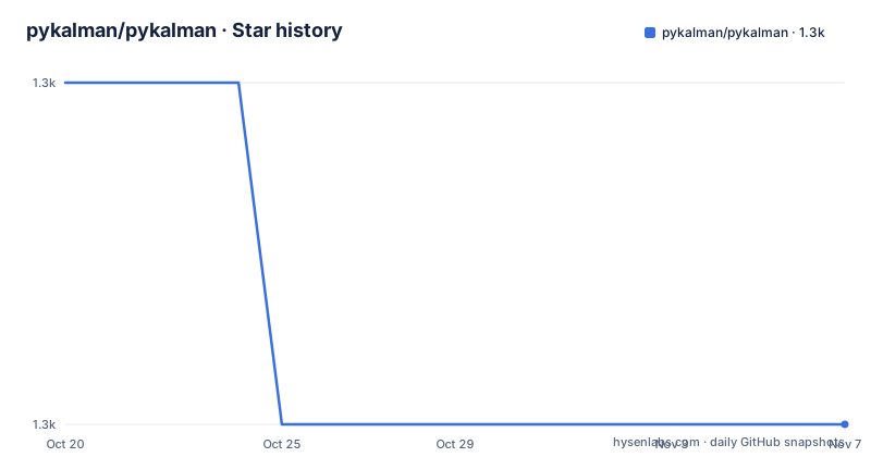
- pykalman/pykalman1,339 ★ · -1
| Repository | 2026-10-20 | 2026-11-07 |
|---|---|---|
| pykalman/pykalman | 1.3k | 1.3k |
-1 Stars in the last 18 days, measured from the daily GitHub snapshot. Compare with other projects
Editorial analysis
Filter, smoother and parameter learning in one object
pykalman describes itself as the dead simple Kalman filter, Kalman smoother and EM library for Python, and the project description is more specific. It is a Python library for Kalman filtering and smoothing, providing efficient algorithms for state estimation in time series, and it includes tools for linear dynamical systems, parameter estimation and sequential data modelling.
The three capabilities are the classic trio. The filter is the online estimator, the smoother is the offline version that uses future observations to revise the past, and the EM algorithm is the machinery for learning the transition and observation matrices when you have data but not a model.
What is unusual for a library of this kind is that all three live on the same object. You construct a filter, call `em` on it to fit the parameters, then call `filter` or `smooth` with the same data. The state estimates come back as pairs, the filtered state means and covariances, and the smoothed state means and covariances, so the shape of the result is the same in both cases and you can compare them directly.
The library was originally created by Daniel Duckworth, and the current maintainers are the pykalman developers, with the project metadata listing an address at gcos.ai. That handover is worth noting, because a scientific library that changes hands is one whose API you should check against the version you pin.
The whole API, in one block
The usage example is short enough to be worth reading closely.
from pykalman import KalmanFilter
import numpy as np
kf = KalmanFilter(transition_matrices = [[1, 1], [0, 1]], observation_matrices = [[0.1, 0.5], [-0.3, 0.0]])
measurements = np.asarray([[1,0], [0,0], [0,1]])  # 3 observations
kf = kf.em(measurements, n_iter=5)
(filtered_state_means, filtered_state_covariances) = kf.filter(measurements)
(smoothed_state_means, smoothed_state_covariances) = kf.smooth(measurements)
The model is specified the way the textbooks do it, with a transition matrix describing how the state moves and an observation matrix describing how the state maps to the measurement. The `em` call with `n_iter=5` runs the expectation maximisation for five iterations and returns a new filter, so the call reads as a pipeline rather than as a configuration step.
Then the same filter is used twice, once for the filtered estimates and once for the smoothed ones. That is the point of the library, that a single model object gives you both the online and the offline answer, and that the offline answer is available whenever you have the whole series.
For a user coming from a statistics course, this will feel like the textbook, which is the highest compliment that can be paid to a scientific library.
Missing data, non-linear dynamics and online filtering
Three extensions are documented, and each addresses a case where the plain filter does not work.
Missing measurements are handled with NumPy's masked arrays rather than with a separate API. You convert the measurements with `ma.asarray`, mark the unobserved timestep with `ma.masked`, and then use the filter exactly as before, including the `em` call.
from numpy import ma
measurements = ma.asarray(measurements)
measurements[1] = ma.masked   # measurement at timestep 1 is unobserved
kf = kf.em(measurements, n_iter=5)
(filtered_state_means, filtered_state_covariances) = kf.filter(measurements)
(smoothed_state_means, smoothed_state_covariances) = kf.smooth(measurements)
Non-linear dynamics are the reason the unscented filter exists, and the API change is that you pass functions instead of matrices.
from pykalman import UnscentedKalmanFilter
ukf = UnscentedKalmanFilter(lambda x, w: x + np.sin(w), lambda x, v: x + v, transition_covariance=0.1)
(filtered_state_means, filtered_state_covariances) = ukf.filter([0, 1, 2])
(smoothed_state_means, smoothed_state_covariances) = ukf.smooth([0, 1, 2])
The online case has its own method, `filter_update`, which takes the previous state estimate and the new measurement and returns the updated one, so a streaming application does not have to refilter the whole series every time a point arrives.
for t in range(1, 3):
    filtered_state_means[t], filtered_state_covariances[t] = \
            kf.filter_update(filtered_state_means[t-1], filtered_state_covariances[t-1], measurements[t])
Taken together, the three extensions cover the three things people most often need and that the plain Kalman filter does not give you.
Square root filters for when the covariance matrix misbehaves
The last documented capability is the numerically robust square root family, imported from a separate namespace.
from pykalman.sqrt import CholeskyKalmanFilter, AdditiveUnscentedKalmanFilter
kf = CholeskyKalmanFilter(transition_matrices = [[1, 1], [0, 1]], observation_matrices = [[0.1, 0.5], [-0.3, 0.0]])
ukf = AdditiveUnscentedKalmanFilter(lambda x, w: x + np.sin(w), lambda x, v: x + v, observation_covariance=0.1)
The reason this exists is a specific numerical failure. The standard filter maintains a covariance matrix and factorises it at each step, and in floating point that factorisation can lose positive definiteness, at which point the filter produces NaNs and does not recover. Working with the square root of the covariance keeps the quantity positive by construction, at the cost of a different algorithm and more work per step.
The design decision here is the separate `pykalman.sqrt` module rather than a flag on the main class. The square root filters are a different implementation with different performance characteristics, and hiding them behind a keyword argument on the same class would have made the two look interchangeable when they are not. The cost of that choice is that you have to know which one you want.
The dependency pins are the most informative part of the metadata
The project metadata constrains the numerical stack tightly, and reading those constraints tells you what kind of library this is.
The runtime dependencies are `numpy<3`, `packaging`, `scikit-base<0.14.0` and `scipy<2.0.0`, and the supported Python range is `>=3.10,<3.15` with classifiers for 3.10 through 3.14.
A library that pins `numpy<3` and `scipy<2` is a library that is careful about the version of the numerical stack it was validated against. That is the right instinct for code that does matrix factorisations, where a change in a linear algebra routine can change results at the level of floating point noise, and where an unvalidated major version can silently break a covariance update. The `scikit-base` dependency is the base class machinery that the filter classes are built on, also bounded below 0.14.
The optional dependency groups show the shape of the project. There is a `tests` extra with pytest, a `dev` extra with pytest and pre-commit, and a `docs` extra with jupyter, Sphinx below 10, numpydoc and matplotlib, and an `all` extra that adds twine for the release. There is also a `numpy1` extra pinning `numpy<2`.
That last extra is a compatibility escape hatch for users who cannot move to numpy 2 yet, and its presence alongside the default `numpy<3` pin tells you the maintainers have to support two numpy generations. The library itself is classified as Development Status 4, Beta, and its intended audience is given as Science and Research, which is a fair self description.
The project around the library
The supporting infrastructure is more organised than most single maintainer libraries manage.
Questions are routed by kind rather than to one inbox. Bug reports and feature requests go to the GitHub issue tracker, usage questions go to a Stack Overflow tag, general discussion goes to Discord, and contributions and development happen in a `dev-chat` channel. There are also scheduled meet-ups, on Fridays at 13 UTC in a dedicated channel, described as meet-ups and collaboration sessions. The stated reason for the arrangement is that they strongly believe in the value of sharing help publicly, so that a wider audience can benefit from it.
The documentation is on Read the Docs and the tutorials live in the repository's `examples/` directory, with `examples/standard/` and `examples/unscented/` as the two families. The repository also carries a `CHANGELOG` and a `CHANGELOG.md`, a `Makefile` with the usual targets, `pip install -e .[all]`, `python -m pytest`, `python -m build .` and `twine upload dist/*` for the release, plus a `build_tools/` directory, a `doc/` directory and a pre-commit configuration.
The release cadence is steady. v0.11.0 was published on 2025-11-27, v0.11.1 on 2025-12-31 and v0.11.2 on 2026-01-31, with the last push to the repository on 2026-04-20. Versions below one and patch releases every few weeks is the profile of a library that is maintained but still finding its final shape, and that is the honest expectation to set.
Where pykalman is the wrong choice
The first wrong case is a very large or very non-linear state space. The filter maintains and factorises a dense covariance matrix at every step, and the unscented variant propagates sigma points through the model on each step, so both costs grow with the dimension of the state. If your state vector has hundreds of dimensions, the arithmetic is the problem and this library is not the answer.
The second wrong case is a problem that is not a linear dynamical system at all. A Kalman filter assumes linear dynamics with Gaussian noise, and while the unscented filter relaxes the linearity, it does not relax the Gaussianity. A system with heavy tailed or multimodal noise needs something else, and no amount of tuning the filter will change that assumption.
The third is a project that needs a much larger ecosystem. pykalman is a focused library with three capabilities, and a team that also needs forecasting, structural time series models, change point detection and plotting wants a statistics package rather than a filter.
The fourth is a production deployment with a hard reproducibility requirement. The library is classified as beta, it depends on a numerical stack it pins rather than owns, and the version of numpy you install can change results at the level of floating point noise in a filter that is already sensitive to conditioning. If a number has to be identical across two machines years apart, that is a stronger requirement than this library makes.
For everything else, the honest summary is that pykalman does one thing, does it in a way that matches the textbook, and covers the three cases people actually hit, the missing observation, the non-linear model and the numerically fragile covariance.
Editorial conclusion
Adopt pykalman if you need state estimation on a time series in Python and want one dependency that covers the filter, the smoother, the non-linear case and the parameter learning, since the alternatives usually mean writing the linear algebra yourself or pulling in a heavier framework. Do not adopt it if your dynamics are deeply non-linear or your state space is very large, because the covariance arithmetic this library performs is dense and the unscented variant multiplies the work per step. Verify first that your numpy and scipy versions are inside the supported range, that the extra you need is installed if you rely on square root filters, and that the API you have in mind matches what the version you pin exposes, since the library is still classified as beta and its dependency pins have moved with each release.
Frequently asked questions
How do I install and use pykalman?
Install it with `pip install pykalman` or `pip install .` from source, on macOS, Linux or Windows 8.1 or higher, with Python 3.10 through 3.14. You create a `KalmanFilter` with transition and observation matrices, run `kf.em(measurements, n_iter=5)` to learn the parameters, then call `kf.filter(measurements)` or `kf.smooth(measurements)` to get the filtered or smoothed state means and covariances.
Does pykalman handle missing measurements?
Yes, through NumPy masked arrays. You convert the measurements with `ma.asarray`, mark the unobserved timestep with `ma.masked`, and then use the filter, the EM routine and the smoother exactly as you would with complete data.
What is the difference between the Kalman filter and the unscented filter in pykalman?
The unscented filter takes functions rather than matrices for the transition and observation, which lets it handle non-linear dynamics, and it is constructed as `UnscentedKalmanFilter(lambda x, w: ..., lambda x, v: ..., transition_covariance=0.1)`. The same filter and smooth calls are used afterwards.
What are the square root filters in pykalman for?
They are the numerically robust variants, imported from `pykalman.sqrt` as `CholeskyKalmanFilter` and `AdditiveUnscentedKalmanFilter`. They work with the square root of the covariance matrix so it stays positive definite in floating point, at the cost of a different algorithm and more work per step.
Which versions of numpy and scipy does pykalman support?
The runtime dependencies are `numpy<3`, `scipy<2.0.0`, `scikit-base<0.14.0` and `packaging`, and there is a `numpy1` extra that pins `numpy<2` for users who have not moved to numpy 2 yet. The library supports Python 3.10 through 3.14.
Official sources
Add this badge to your README
If you maintain this project, the badge below links readers to this analysis and shows its maintenance status from the daily GitHub snapshot. Paste the markdown into your README; add ?metric=license or ?metric=stars to the image URL for a different field.

[](https://hysenlabs.com/projects/pykalman-pykalman)Star history chart for your README
[](https://hysenlabs.com/projects/pykalman-pykalman)Was this useful?