dynamax puts state space models, filtering and learning in one JAX library
A Python package for probabilistic state space modeling with JAX
At a glance
- What is it?
- Dynamax is a Python library for probabilistic state space models written in JAX, covering hidden Markov models, linear, nonlinear and generalized Gaussian state space models, with inference algorithms and an object oriented model layer on top. It is a Probabilistic Machine Learning project, MIT licensed, and it plugs into optax and Blackjax for parameter learning.
- Who is it for?
- dynamax is worth adopting if you are working with time series with latent structure and you want the same code to run on a CPU and on an accelerator, because the inference algorithms are pure functions that JAX can differentiate and vectorise, and the model classes cover the HMM, linear, nonlinear and generalized Gaussian cases in one API.
- Can I use it commercially?
- Yes. MIT is a permissive licence: you can use, modify and sell software built on it, as long as you keep its copyright and licence notices.
- Is it still maintained?
- Yes. The repository last received commits 6 days ago.
- What is it written in?
- Mainly Python, according to GitHub's language statistics.
Answers come from the project's GitHub data, last synced on November 7, 2026, and from our analysis. They are not legal advice.
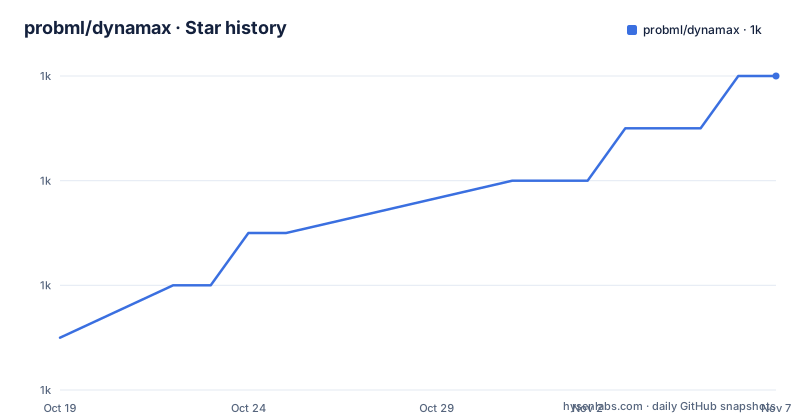
Star history
- probml/dynamax1,024 ★ · +5
| Repository | 2026-10-19 | 2026-11-07 |
|---|---|---|
| probml/dynamax | 1k | 1k |
5 Stars in the last 19 days, measured from the daily GitHub snapshot. Compare with other projects
Editorial analysis
A library for the model, not a framework around one
Dynamax is a library for probabilistic state space models, written in JAX, and the project description is precise about what it covers. It has code for inference, meaning state estimation, and learning, meaning parameter estimation, in a variety of state space models: hidden Markov models, linear Gaussian state space models which are also known as linear dynamical systems, nonlinear Gaussian state space models, and generalized Gaussian state space models with non-Gaussian emission models.
The structure of the library is stated as a set of core, functionally pure, low-level inference algorithms, plus a set of model classes providing a more user-friendly, object-oriented interface. That two layer split is the design decision that matters.
The core layer is functionally pure, which in JAX means the algorithms are ordinary functions of their inputs, with no hidden state and no in-place mutation. That is what makes them differentiable, which is what makes them composable with autodiff, and it is what allows the same filtering routine to be used inside a larger model.
The model layer is where the ergonomics live. A GaussianHMM object knows its own parameterisation, knows how to initialise itself, how to sample from itself and how to fit itself, and the inference algorithms are called on it rather than being configured by hand.
The audience is a probabilistic modelling researcher or an engineer with a time series problem who is already using JAX. The project comes from the Probabilistic Machine Learning group, the same group behind the pml-book, and it is compatible with other libraries in the JAX ecosystem, with optax used for estimating parameters by stochastic gradient descent and Blackjax used for computing the parameter posterior by Hamiltonian Monte Carlo or sequential Monte Carlo.
The licence is MIT, the package requires Python 3.10 or newer, and it is a published PyPI package with a JOSS paper, doi 10.21105/joss.07069, that summarises the library.
What a state space model is, and why the library exists
The readme explains the model before the API, and the explanation is the justification for the library's design.
A state space model is a partially observed Markov model in which the hidden state, z_t, evolves over time according to a Markov process, possibly conditional on external inputs, controls or covariates, u_t, and generates an observation, y_t. The joint distribution is given in a form the library restricts to discrete time systems, and the readme names the two pieces: p(z_t given z_t-1, u_t) is the transition or dynamics model, and p(y_t given z_t, u_t) is the observation or emission model. The inputs u_t are optional, and the observation model may have autoregressive dependencies, in which case it is written with the past observations as well.
Then comes the point of the whole exercise. We assume that we see the observations and want to infer the hidden states, either using online filtering, computing p(z_t given y_1:t), or offline smoothing, computing p(z_t given y_1:T). We may also be interested in predicting future states or future observations at a forecast horizon h. And the note that carries the argument for state space models in general: by using a hidden state to represent the past observations, the model can have effectively infinite memory, unlike a standard autoregressive model.
That last sentence is the honest motivation. A Kalman filter carries the entire past in its mean and covariance, and an HMM carries it in the state distribution, and that is what makes these models different from a deep sequence model with a fixed context window.
The readme also points at the two books that cover the mathematics, Kevin Murphy's Machine Learning: Advanced Topics from MIT Press in 2023, and Bayesian Filtering and Smoothing, second edition, by Särkkä and Svensson from Cambridge University Press in 2023. For a library that implements these algorithms, the books are the reference for why the algorithms are shaped the way they are.
The Gaussian HMM example is the whole API in twenty lines
The example in the readme is a Gaussian emission HMM, and it is worth reading closely because it shows the shape of the entire library.
import jax.numpy as jnp
import jax.random as jr
import matplotlib.pyplot as plt
from dynamax.hidden_markov_model import GaussianHMM

key1, key2, key3 = jr.split(jr.PRNGKey(0), 3)
num_states = 3
emission_dim = 2
num_timesteps = 1000

# Make a Gaussian HMM and sample data from it
hmm = GaussianHMM(num_states, emission_dim)
true_params, _ = hmm.initialize(key1)
true_states, emissions = hmm.sample(true_params, key2, num_timesteps)

# Make a new Gaussian HMM and fit it with EM
params, props = hmm.initialize(key3, method="kmeans", emissions=emissions)
params, lls = hmm.fit_em(params, props, emissions, num_iters=20)

# Plot the marginal log probs across EM iterations
plt.plot(lls)
plt.xlabel("EM iterations")
plt.ylabel("marginal log prob.")

# Use fitted model for posterior inference
post = hmm.smoother(params, emissions)
print(post.smoothed_probs.shape) # (1000, 3)
Four things happen. The model is constructed with its dimensions, 3 states and 2 dimensional Gaussian emissions. It is initialised with a PRNG key, which returns the parameters and the associated properties. It is sampled from to produce ground truth states and emissions. A second model is initialised using the emissions, with the method set to kmeans, so the initialisation is data aware rather than random, and then fitted with expectation maximisation for 20 iterations, returning the fitted parameters and a list of marginal log probabilities. Finally the fitted model is used for posterior inference, and the smoother returns an object whose smoothed_probs attribute has shape (1000, 3), one probability per state per timestep.
That shape is the point of the whole exercise. A smoother that runs 1000 timesteps over 3 states and returns the full posterior state matrix is something you can put straight into a loss function, because everything in the library is a pure JAX function and therefore differentiable.
Batching comes from vmap, not from a data loader
The second example in the readme shows the other half of the story, and it is short.
from functools import partial
from jax import vmap

num_seq = 200
batch_true_states, batch_emissions = \
    vmap(partial(hmm.sample, true_params, num_timesteps=num_timesteps))(
        jr.split(key2, num_seq))
print(batch_true_states.shape, batch_emissions.shape) # (200,1000) and (200,1000,2)

# Make a new Gaussian HMM and fit it with EM
params, props = hmm.initialize(key3, method="kmeans", emissions=batch_emissions)
params, lls = hmm.fit_em(params, props, batch_emissions, num_iters=20)
The readme puts it as JAX allowing you to easily vectorize these operations with vmap, so you can sample and fit to a batch of emissions. 200 sequences of 1000 timesteps with 2 dimensional emissions, sampled in one vmapped call and fitted in one EM run.
That is the practical difference between this library and a conventional one. There is no DataLoader and no batch size argument. You write the computation for one sequence, and vmap lifts it, and JAX decides whether that means vectorised CPU code, a GPU kernel, or a jitted compiled function. The cost of that freedom is that the shape discipline is on you, and the cost of a conventional framework is that you are working inside its model of the world.
The runtime dependencies listed in the project metadata reflect the same design: jax and jaxlib, tfp-nightly, optax, jaxtyping for the type annotations, fastprogress for progress bars, typing-extensions and numpy. The optional notebook extra adds matplotlib, seaborn, flax, blackjax, graphviz, scipy and scikit-learn, which is the set of things you need to draw, fit with modern gradient based methods and read the docs.
Parameter learning is where the ecosystem does the work
The readme is clear that dynamax does not own the whole task. It reuses the rules from the markdownlint-like separation of concerns, and here it is stated as compatibility with other libraries in the JAX ecosystem.
optax is used for estimating parameters using stochastic gradient descent, and Blackjax is used for computing the parameter posterior using Hamiltonian Monte Carlo or sequential Monte Carlo. So the division of labour is: dynamax provides the likelihood and the inference algorithms, optax provides the optimiser, and Blackjax provides the sampler.
That is a bigger claim than it sounds, because it means the same model can be fitted three ways. Expectation maximisation is built in and is the natural choice for a maximum likelihood fit on an HMM. Stochastic gradient descent through optax opens the door to a deep emission model, because the gradient of the marginal log likelihood can be taken through the same inference code. And a Blackjax sampler gives you a posterior over the parameters rather than a point estimate, which is what you want when the data is thin or the identifiability is poor.
The wider Probabilistic Machine Learning ecosystem is present as well. There is an extension, sts-jax, for structural time series models, and bayeux, from the JAX ML group, is shown performing Bayesian inference for the parameters of a state space model, which is the canonical use of a sampler with a state space likelihood.
The upshot is that dynamax is the model and inference layer, and the rest of the JAX ecosystem is the learning layer. For a user who wants everything in one framework, that is a feature. For a user who already has a working pipeline with optax and a sampler, it means the state space model can drop into it without a rewrite.
Maintenance state, and the nightly dependency to watch
The repository is not archived, and the last push was on 2026-10-13, the same day as the release 1.0.3. Before that came 1.0.2 on 2026-06-25 and 1.0.1 on 2025-05-10, so the project is on a stable 1.0 line and shipping patch releases.
The version number is generated rather than written. The project metadata declares the version as dynamic, and setup.py gets it from versioneer, with a versioneer.py at the repository root, which means the version follows the git tags rather than a value edited in a file. The CITATION.cff file at the root is there for the same reason, so a paper citation resolves to a commit.
The dependency worth flagging is tfp-nightly. The runtime dependency list includes a nightly build of TensorFlow Probability, which means the library is tracking a moving target for its probability primitives. That is a reasonable choice inside the JAX ecosystem, where a stable release would lag the JAX version, and it is also a choice that can break a pinned environment on an unrelated day. If you deploy this, pin the environment carefully, and expect to test a build after each JAX upgrade rather than assuming a version bump is inert.
The rest of the metadata is ordinary good practice. The extras are named for their purpose, notebooks, doc, test and dev, and the test extra includes pytest, pytest-cov, coverage and codecov, and interrogate, which is a tool that measures docstring coverage. The readme badges show a test workflow and a separate interrogate workflow, so the docstrings are checked like the tests are.
The documentation itself is split between the JOSS paper, which the readme recommends as a high level summary, and the site at probml.github.io/dynamax, which carries the tutorials and the API reference. The package is by the authors Scott Linderman, Peter Chang, Giles Harper-Donnelly, Aleyna Kara, Xinglong Li and Kevin Murphy, and is maintained by Scott Linderman.
Editorial conclusion
dynamax is worth adopting if you are working with time series with latent structure and you want the same code to run on a CPU and on an accelerator, because the inference algorithms are pure functions that JAX can differentiate and vectorise, and the model classes cover the HMM, linear, nonlinear and generalized Gaussian cases in one API. It is the wrong choice if your model is a deep sequence model, since a recurrent network is usually the better fit for long range dependencies than a linear dynamical system. Before you depend on it, check that your JAX version matches the pinned jaxlib, note that the runtime dependencies include a nightly TensorFlow Probability build, and note that the current release is 1.0.3 from 2026-10-13 with the repository pushed to on the same day.
Frequently asked questions
What models does dynamax support?
It has code for inference and learning in hidden Markov models, linear Gaussian state space models also known as linear dynamical systems, nonlinear Gaussian state space models, and generalized Gaussian state space models with non-Gaussian emission models. The library is organised as a set of functionally pure low-level inference algorithms plus object-oriented model classes on top.
How do I install dynamax?
From PyPI with pip install dynamax, or pip install dynamax[notebooks] for the demo notebook dependencies, or pip install git+https://github.com/probml/dynamax.git for the development branch. Developers clone the repository and run pip install -e '.[dev]' to get the test and documentation dependencies as well.
How do I fit a model in dynamax and run inference on it?
You initialise the model with a PRNG key, optionally using the emissions with method="kmeans" for a data aware start, fit it with fit_em for a number of iterations, and then call the smoother to get posterior state probabilities, for example hmm.smoother(params, emissions) returning an object whose smoothed_probs has shape (1000, 3) for three states over a thousand timesteps.
What does dynamax use for parameter estimation?
The library is compatible with the wider JAX ecosystem: optax is used for estimating parameters with stochastic gradient descent, and Blackjax is used for computing the parameter posterior with Hamiltonian Monte Carlo or sequential Monte Carlo. A separate project, bayeux, demonstrates Bayesian inference for state space model parameters.
How do I run the dynamax tests?
With pytest. The readme gives pytest dynamax to run all tests, pytest dynamax/hmm/inference_test.py to run a specific test file, and pytest -k lgssm to select tests by name. The package requires Python 3.10 or newer.
Official sources
Add this badge to your README
If you maintain this project, the badge below links readers to this analysis and shows its maintenance status from the daily GitHub snapshot. Paste the markdown into your README; add ?metric=license or ?metric=stars to the image URL for a different field.

[](https://hysenlabs.com/projects/probml-dynamax)Star history chart for your README
[](https://hysenlabs.com/projects/probml-dynamax)Was this useful?