samila: A Generative Art Generator Where Points Follow a Random Formula
A Generative Art Generator
At a glance
- What is it?
- Samila is a Python library that plots thousands of points, each positioned by a mathematical function whose parameters are random, so no two images are the same. You supply one or two functions, choose how they are compared, pick a projection, a marker, a rotation, a range and a colour scheme, and the library draws it with matplotlib.
- Who is it for?
- Samila fits a Python developer who wants to produce a large number of distinct plots quickly, for teaching, for wallpapers, for album art or as input to something else, because the point generation, the comparison mode and the styling are all parameterised in one place.
- Can I use it commercially?
- Yes. MIT is a permissive licence: you can use, modify and sell software built on it, as long as you keep its copyright and licence notices.
- Is it still maintained?
- Yes. The repository last received commits 4 days ago.
- What is it written in?
- Mainly Python, according to GitHub's language statistics.
Answers come from the project's GitHub data, last synced on November 6, 2026, and from our analysis. They are not legal advice.
Star history
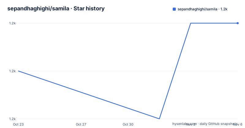
- sepandhaghighi/samila1,189 ★ · +1
| Repository | 2026-10-23 | 2026-11-06 |
|---|---|---|
| sepandhaghighi/samila | 1.2k | 1.2k |
1 Stars in the last 14 days, measured from the daily GitHub snapshot. Compare with other projects
Editorial analysis
Thousands of Points From One Random Formula
Samila is a generative art generator written in Python, and the description in the package metadata explains the mechanism in one paragraph. Samila lets you create images based on many thousand points, the position of every single point is calculated by a formula, which has random parameters, and because of the random numbers every image looks different.
That is the whole model, and it is a good one. A function maps two coordinates to a value, the value is turned into a point, and thousands of points make a picture. The randomness is inside the formula rather than in the coordinates, which is why the pictures have structure: the same function evaluated many times over a grid of inputs produces a shape, and the random parameters give each run a different shape of the same family.
The library is a layer over matplotlib rather than a renderer of its own, and the requirements file says so plainly, with matplotlib at 3.0.0 or newer, art at 1.8 or newer, and Pillow at 6.2 or newer for image handling.
The practical appeal is speed of iteration. Writing a plotting program by hand to explore a family of functions is a few lines of code, but exploring variations across modes, projections and markers is the kind of combinatorial thing a library is for.
Your Two Functions and the Seed That Identifies the Result
The simplest use involves no functions at all. The Magic example in the README is four lines:
>>> import matplotlib.pyplot as plt
>>> from samila import GenerativeImage
>>> g = GenerativeImage()
>>> g.generate()
>>> g.plot()
>>> plt.show()
With no functions supplied, the library uses its own. The Basic example shows what supplying your own looks like, with two functions of x and y and the image constructed from them:
>>> g = GenerativeImage(f1, f2)
>>> g.generate()
>>> g.plot()
>>> g.seed
188781
>>> plt.show()
The seed attribute is the part to notice. Every generated image reports the seed it came from, which is the identifier you need to find that image again or to reason about it later, and it is printed in the examples after every generation.
The function generation seed is separately controllable, and the README notes that you can change it with the func_seed parameter in GenerativeImage. That is the distinction to keep straight. The seed reported by the image is the result seed, and the func_seed is the seed of the random parameters baked into the function, and pinning the second one is how you get a stable family of shapes rather than a fresh family on every run.
Generation Modes Decide Which Curve Is Compared With Which
The generation mode is the main structural choice, and the library exposes a large set of them.
The supported modes are F1_VS_F2, F2_VS_F1, F1_VS_INDEX, F2_VS_INDEX, INDEX_VS_F1, INDEX_VS_F2, F1_VS_X1, F1_VS_X2, F2_VS_X1, F2_VS_X2, X1_VS_F1, X1_VS_F2, X2_VS_F1, X2_VS_F2, F1F2_VS_F1, F1F2_VS_F2, F1_VS_F1F2, F2_VS_F1F2 and RANDOM, and the default is F1_VS_F2.
The naming scheme is worth decoding rather than skipping, because it tells you the shape of the result. The mode names two things being compared, and the token on the left of VS is the value used for the y coordinate while the one on the right supplies the x coordinate, and the tokens are the two functions F1 and F2, the point index INDEX, and the two x coordinates X1 and X2. So F1_VS_F2 plots the first function against the second, and F1_VS_INDEX plots the first function against the position of the point, which produces a curve rather than a scatter, and RANDOM picks a mode at random.
The combinations that use INDEX, X1 and X2 are what make the library more than a two function plotter, because the same function produces a different picture depending on what it is plotted against. That is a real design idea, and the mode list is the documentation of it.
Projections and Markers Are the Visual Vocabulary
Two enums control how the points are drawn, and both are set on the plot call rather than the generate call, which is a detail that matters when you are iterating.
The projections are RECTILINEAR, POLAR, AITOFF, HAMMER, LAMBERT, MOLLWEIDE and RANDOM, with RECTILINEAR as the default. These are the map projections applied to the coordinate system, and the list is the standard set of world projections. Applying a polar projection to a scatter of points turns a curve into a spiral of points around the pole, which is the cheapest way to make a familiar picture look unfamiliar.
The markers are a much longer list, POINT, PIXEL, CIRCLE, TRIANGLE_DOWN, TRIANGLE_UP, TRIANGLE_LEFT, TRIANGLE_RIGHT, TRI_DOWN, TRI_UP, TRI_LEFT, TRI_RIGHT, OCTAGON, SQUARE, PENTAGON, PLUS, PLUS_FILLED, STAR, HEXAGON_VERTICAL, HEXAGON_HORIZONTAL, X, X_FILLED, DIAMOND, DIAMON_THIN, VLINE, HLINE and RANDOM, with POINT as the default. The marker is passed with a spot size:
>>> g = GenerativeImage(f1, f2)
>>> g.generate()
>>> g.plot(marker=Marker.CIRCLE, spot_size=10)
>>> g.seed
448742
The size of the marker matters as much as its shape at high point counts, because a plot of thousands of points with large markers is a solid field rather than a scatter, and that is often the difference between an image and a chart.
Rotation, Range and Colour Are the Remaining Knobs
Three more parameters complete the control surface, and each solves a specific problem.
Rotation is applied to the image in degrees, and the README puts it plainly: you can even rotate your art by using the rotation parameter, enter your desired rotation for the image in degrees and you will have it. The default is 0.
The range is the domain over which the function is evaluated, and it is set on generate rather than on plot:
>>> g = GenerativeImage(f1, f2)
>>> g.generate(start=-2*math.pi, step=0.01, stop=0)
>>> g.plot()
>>> g.seed
234752
The default range is negative pi to pi, and the step parameter is the increment across that range, so the step is what determines the point count together with the range length. Narrowing the range to negative two pi to zero with a step of 0.01 produces a quarter of the points of the default and a different shape.
Colour is the last of the three, with a color and a bgcolor, and the defaults are black and white respectively. The supported colours are in a VALID_COLORS list, and the parameters accept a colour name, for example color="yellow", or an RGB or RGBA value. The colour parameters are independent of the projection, so you can set a polar projection with a yellow foreground and a black background in the same call.
Installing From PyPI, Source or Conda
There are three documented installation routes, and the README is specific about each.
From PyPI, the instruction is to run pip install samila==1.6, with a link to the Python Packaging User Guide. From source, you download the Version 1.6 archive or the latest source from the dev branch and run pip install . in the unpacked directory. And from Conda, the command is conda install -c sepandhaghighi samila, with a link to the Conda documentation.
The setup module reflects the same care about metadata. The description is read from the README and the CHANGELOG so that the long description on the package index matches the repository, with a fallback minimal description if either file cannot be read, and the requirements are read from requirements.txt rather than being duplicated in the setup file. The package supports Python 3.7 and newer, and the version is set to 1.6 in the setup file to match the release.
The distribution channels are also broad. There is a PyPI badge, an Anaconda badge, a Colab badge for running it in a notebook, and a Discord badge for the community channel.
For anyone who wants to try it without installing anything, the examples directory holds a bulk.ipynb notebook and a demo.ipynb notebook, and the README's own examples are written as pycon sessions, which is the format that makes them readable as documentation.
The Repository Layout and the Release Line
The repository is a conventional Python package with the project tooling beside it. There is the samila/ package itself, an examples/ directory with the two notebooks, an otherfiles/ directory holding the logo and the example images used in the README, and a test/ directory. The configuration is pytest.ini for the tests, codecov.yml and .coveragerc for coverage, requirements.txt and dev-requirements.txt for the dependencies, and a pair of autopep8 scripts for formatting.
The quality signals are the usual set of badges. There is a codecov badge, a code quality grade from Codacy, a CodeFactor badge, and a CI badge for both the master and the dev branch, with the branch table in the README showing that master and dev are tested in parallel.
The release history is a small version sequence with dates, 1.6 from 2025-07-16, 1.5 from 2025-01-22 and 1.4 from 2024-11-20, and the repository also carries a CHANGELOG.md, an AUTHORS.md and a SECURITY.md, which is more governance than most library of this size has.
The site for the project is samila.site, the primary language of the repository is Python, the licence is MIT, the repository is not archived, and the last push was on 2026-10-05.
Editorial conclusion
Samila fits a Python developer who wants to produce a large number of distinct plots quickly, for teaching, for wallpapers, for album art or as input to something else, because the point generation, the comparison mode and the styling are all parameterised in one place. It is a poor fit for a reproducible art pipeline, since the seed changes on every run and the functions use a random uniform inside the formula itself, so the same code does not give you the same picture twice unless you pin the function generation seed. Before using it, note that the seed attribute is reported per image, which is the identifier you need if you want to regenerate a specific result, and that the default range is negative pi to pi with a step of 0.01, which gives a dense result at the default point count. The project is MIT licensed, the current release is 1.6 from 2025-07-16, and the last push was on 2026-10-05.
Frequently asked questions
How does Samila generate an image?
It creates images based on many thousand points, where the position of every single point is calculated by a formula that has random parameters, so because of the random numbers every image looks different. The library is a layer over matplotlib and the art and Pillow libraries.
How do I install Samila?
From PyPI with `pip install samila==1.6`, from source by downloading the version or the dev branch archive and running `pip install .`, or from Conda with `conda install -c sepandhaghighi samila`. The package requires Python 3.7 or newer.
What are the generation modes in Samila?
The supported modes are F1_VS_F2, F2_VS_F1, F1_VS_INDEX, F2_VS_INDEX, INDEX_VS_F1, INDEX_VS_F2, F1_VS_X1, F1_VS_X2, F2_VS_X1, F2_VS_X2, X1_VS_F1, X1_VS_F2, X2_VS_F1, X2_VS_F2, F1F2_VS_F1, F1F2_VS_F2, F1_VS_F1F2, F2_VS_F1F2 and RANDOM, with F1_VS_F2 as the default. The names describe what is plotted against what.
Which projections and markers does Samila support?
The projections are RECTILINEAR, POLAR, AITOFF, HAMMER, LAMBERT, MOLLWEIDE and RANDOM, with RECTILINEAR as the default. The markers range from POINT and PIXEL through CIRCLE, the triangles, OCTAGON, SQUARE, PENTAGON, PLUS, STAR, the hexagons, X, DIAMOND, VLINE and HLINE to RANDOM, with POINT as the default.
Can I reproduce the same Samila image later?
Each generated image reports its seed through the seed attribute, and the README notes that the function generation seed can be changed with the func_seed parameter of GenerativeImage. The default range is negative pi to pi, the step defaults to 0.01, and rotation defaults to 0.
Official sources
Add this badge to your README
If you maintain this project, the badge below links readers to this analysis and shows its maintenance status from the daily GitHub snapshot. Paste the markdown into your README; add ?metric=license or ?metric=stars to the image URL for a different field.

[](https://hysenlabs.com/projects/sepandhaghighi-samila)Star history chart for your README
[](https://hysenlabs.com/projects/sepandhaghighi-samila)Was this useful?